7 Part 7 (On your own)
7.1 Modeling bird stopover distributions
This last section is to quickly model bird stopover distributions using Boosted Regression Trees. You will use a subset of data from three radars along the mid-Atlantic USA. The data have already been processed to produce the mean Vertically-Integrated Reflectivity (meanVIR) and coefficient of variation of VIR (cvVIR) in units of cm2 per hectare for autumn stopover density of land birds pooled across years from 2008-2014. The data were aggregated to a 1km x 1km resolution grid and subsetted to cells separated by 5km to improve spatial independence of the data. There are several explanatory variables also summarized for the grid cells that include:
`UTMX` - Easting coordinate

`UTMY` - Northing coordinate

`elev` - elevation in meters above sea level

`dcoast` - distance from the nearest coastline in km

`pwood` - proportion of evergreen pine forest cover in grid cell

`emmarsh` - proportion of emergent marsh cover in grid cell

`hwood` - proportion of deciduous hardwood forest cover in grid cell

`urban` - proportion of urban cover in grid cell

`ag` - proportion of agricultural land cover in grid cell

`ndvimean` - mean seasonal Normalized Difference Vegetation Index

`ndvistd` - standard deviation of NDVI

`near_radar` - proximity to the nearest radar in m
Let’s start by getting some libraries and functions set up.
reqPackages <- c('mgcv','fields','dismo','spdep',"RColorBrewer","plotrix")
get.packages <- reqPackages[!(reqPackages %in% installed.packages()[,"Package"])]
if(length(get.packages)>0) install.packages(get.packages,dependencies = TRUE)

library(mgcv)
library(fields)
library(dismo)
library(spdep)
library(RColorBrewer)
library(plotrix)

##Function to flatten a correlation matrix into a data frame
flattenCorrMatrix <- function(cormat) {
  ut <- upper.tri(cormat)
  data.frame(
    row = rownames(cormat)[row(cormat)[ut]],
    column = rownames(cormat)[col(cormat)[ut]],
    cor  =(cormat)[ut]

  )
}
##Function for resetting plotting parameters
resetPar <- function() {
  dev.new()
  op <- par(no.readonly = TRUE)
  dev.off()
  op
}
OK. Now let’s load up the data and check for multicollinearity among variables.
setwd(OUT)
data<-read.csv("bird_density_1kmgrid_subset.csv")
##Check for multicollinearity
cormatrix<-cor(data)
b<-flattenCorrMatrix(cormatrix)
b = b[order(b$cor),]
b
## row column cor
## 13 UTMX dcoast -0.660281926
## 9 UTMX elev -0.568684073
## 55 urban ag -0.480984604
## 1 meanVIR cvVIR -0.471253500
## 65 urban ndvimean -0.456862403
## 45 hwood urban -0.454107332
## 76 urban ndvistd -0.422026577
## 63 emmarsh ndvimean -0.384281051
## 11 meanVIR dcoast -0.349726905
## 54 hwood ag -0.342681560
## 73 pwood ndvistd -0.313515073
## 27 dcoast emmarsh -0.268047685
## 7 meanVIR elev -0.259619483
## 70 UTMY ndvistd -0.239895868
## 49 UTMY ag -0.228294034
## 68 cvVIR ndvistd -0.218279726
## 43 pwood urban -0.217716027
## 85 pwood near_radar -0.211926385
## 48 UTMX ag -0.207225835
## 36 emmarsh hwood -0.197652896
## 26 elev emmarsh -0.185540343
## 52 pwood ag -0.178216438
## 58 UTMX ndvimean -0.162907321
## 69 UTMX ndvistd -0.157243526
## 57 cvVIR ndvimean -0.155895351
## 53 emmarsh ag -0.150611389
## 30 cvVIR hwood -0.147769079
## 44 emmarsh urban -0.146133101
## 81 UTMX near_radar -0.138298338
## 37 meanVIR urban -0.128589504
## 16 meanVIR pwood -0.118121145
## 14 UTMY dcoast -0.110878523
## 47 cvVIR ag -0.098076862
## 20 elev pwood -0.092663404
## 21 dcoast pwood -0.072153288
## 28 pwood emmarsh -0.067489177
## 72 dcoast ndvistd -0.060408936
## 78 ndvimean ndvistd -0.060178225
## 59 UTMY ndvimean -0.057024256
## 3 cvVIR UTMX -0.053009199
## 31 UTMX hwood -0.048767322
## 32 UTMY hwood -0.042097558
## 41 elev urban -0.039051484
## 25 UTMY emmarsh -0.036744665
## 89 ag near_radar -0.034941343
## 46 meanVIR ag -0.020625505
## 4 meanVIR UTMY -0.014910710
## 86 emmarsh near_radar -0.007550344
## 22 meanVIR emmarsh -0.003898394
## 19 UTMY pwood -0.001314135
## 90 ndvimean near_radar 0.005538626
## 42 dcoast urban 0.025559503
## 23 cvVIR emmarsh 0.032346303
## 71 elev ndvistd 0.032594312
## 87 hwood near_radar 0.045453310
## 66 ag ndvimean 0.052631811
## 91 ndvistd near_radar 0.053568245
## 51 dcoast ag 0.066641052
## 88 urban near_radar 0.073751109
## 35 pwood hwood 0.074206857
## 10 UTMY elev 0.081053876
## 34 dcoast hwood 0.086336336
## 74 emmarsh ndvistd 0.086750074
## 79 meanVIR near_radar 0.087946351
## 50 elev ag 0.094285697
## 39 UTMX urban 0.095125598
## 33 elev hwood 0.106928100
## 17 cvVIR pwood 0.114340312
## 8 cvVIR elev 0.125258116
## 80 cvVIR near_radar 0.125643627
## 18 UTMX pwood 0.136885520
## 24 UTMX emmarsh 0.154395008
## 38 cvVIR urban 0.155108682
## 56 meanVIR ndvimean 0.155463442
## 82 UTMY near_radar 0.156599689
## 84 dcoast near_radar 0.157354656
## 5 cvVIR UTMY 0.163427334
## 75 hwood ndvistd 0.173566982
## 61 dcoast ndvimean 0.197846183
## 67 meanVIR ndvistd 0.228904439
## 60 elev ndvimean 0.236595646
## 29 meanVIR hwood 0.239859255
## 12 cvVIR dcoast 0.258564880
## 2 meanVIR UTMX 0.258823992
## 40 UTMY urban 0.267292868
## 62 pwood ndvimean 0.267336954
## 83 elev near_radar 0.350132218
## 77 ag ndvistd 0.386065559
## 15 elev dcoast 0.550849402
## 64 hwood ndvimean 0.598296970
## 6 UTMX UTMY 0.614191000Nothing too strongly correlated (|r|>0.7). Let’s move on.
Let’s plot the data. It’s not too fancy but gives us an impression of the bird distribution patterns. Hotter color = higher bird density.
dataproj<-st_as_sf(data, coords = c("UTMX", "UTMY"))
st_crs(dataproj)<-26918 #UTM 18N
gbmap <- rast(gmap(dataproj, type = "satellite",map_key="AIzaSyDZohZKjKe4J14NrZBxbf58HV097oEzgdE"))
## Warning: [rast] unknown extentdataproj<-st_transform(dataproj, crs(gbmap))# Google Maps are in Mercator projection. This projects the points to that projection to enable mapping
palette(brewer.pal(n = 9, name = "OrRd"))
plot(gbmap)
points(dataproj, col = plotrix:::rescale(dataproj$meanVIR, c(1, 9)),pch=20)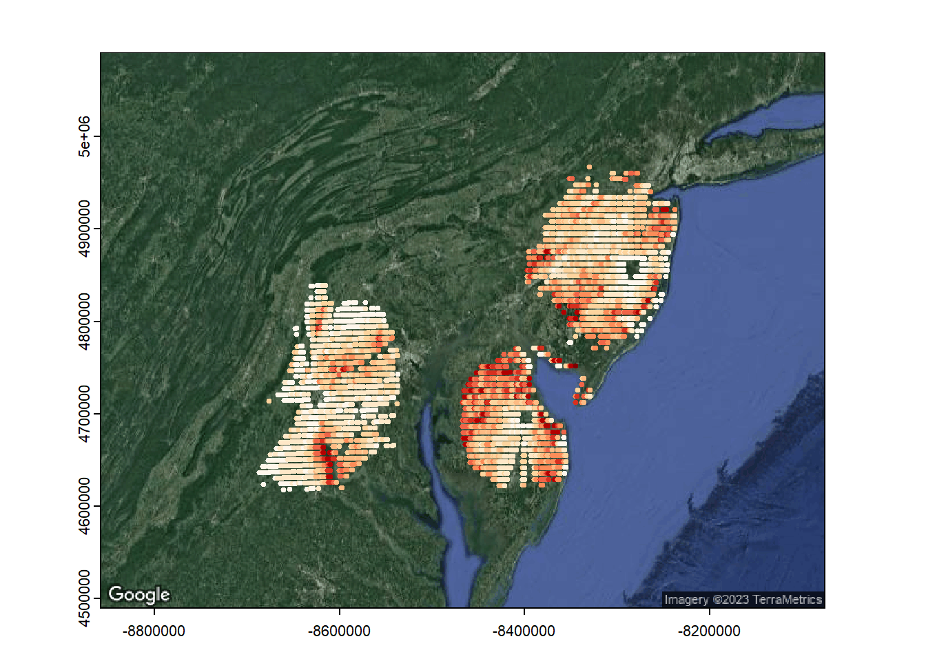
Let’s model VIR with a Boosted Regression Tree. We will set the tree complexity to 1 to first examine main effects with no interactions among covariates. Note that no data transformations are performed. This is because assumptions of normality of data are not required.
The boosting process iteratively tunes the models to more closely fit the training data. We will set the bag.fraction to 0.5, which means 50% of the data will be used to train the models while the remainder are used to cross-validate the models. The boosting continues until the point of minimal holdout deviance is reached. Once the deviance starts to creep back up, it means we are starting to overfit the model. We want to aim for around 1000 trees before reaching the stopping point. You can adjust the learning rate to tune how many trees are run.
brt_model  <- gbm.step(data=data,
                       gbm.x = c("elev","near_radar","pwood","hwood","urban","ndvimean","ndvistd","dcoast","ag","emmarsh"),
                       gbm.y = "meanVIR",
                       family="gaussian",
                       tree.complexity = 5, #set to 1 for no interactions - set >1 for interactions
                       learning.rate = 0.1,
                       bag.fraction = 0.5,n.trees=100)
## Loading required namespace: gbm##
##
## GBM STEP - version 2.9
##
## Performing cross-validation optimisation of a boosted regression tree model
## for NA and using a family of gaussian
## Using 3472 observations and 10 predictors
## creating 10 initial models of 100 trees
##
## folds are unstratified
## total mean deviance = 0.2019
## tolerance is fixed at 2e-04
## ntrees resid. dev.
## 100 0.0969
## now adding trees...
## 200 0.0907
## 300 0.0886
## 400 0.0877
## 500 0.0869
## 600 0.0869
## 700 0.0864
## 800 0.0867
## 900 0.0868
## 1000 0.0868
## 1100 0.0869
## 1200 0.087
## 1300 0.0866
## 1400 0.0866
## 1500 0.0869
## 1600 0.0868
## 1700 0.0869
## 1800 0.087
## 1900 0.087
## 2000 0.0873
## 2100 0.0873
## 2200 0.0877## fitting final gbm model with a fixed number of 700 trees for NA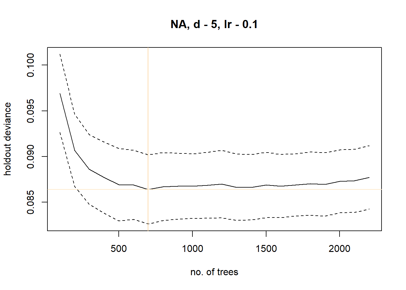
##
## mean total deviance = 0.202
## mean residual deviance = 0.035
##
## estimated cv deviance = 0.086 ; se = 0.004
##
## training data correlation = 0.913
## cv correlation =  0.757 ; se = 0.008
##
## elapsed time -  0.93 minutes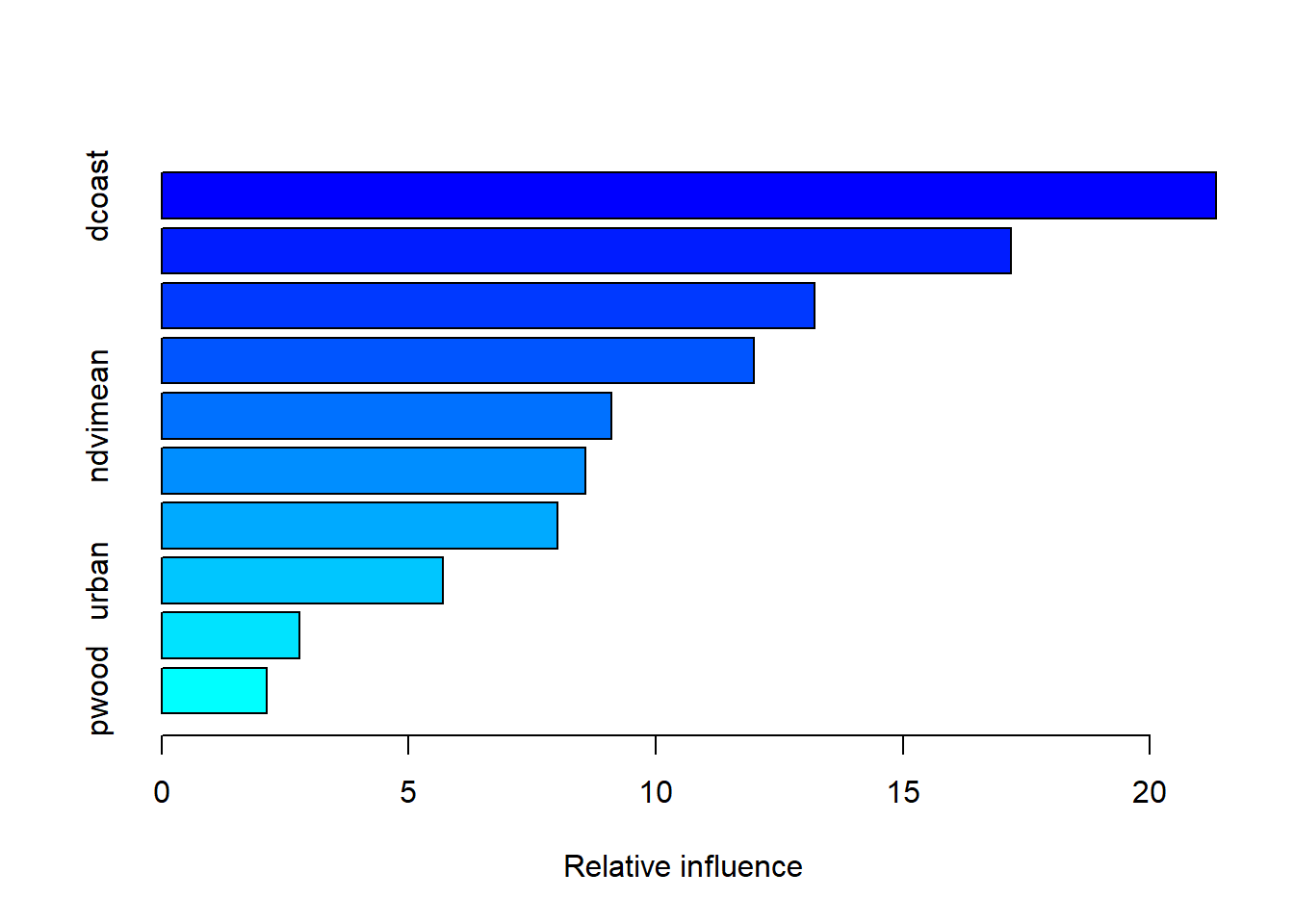
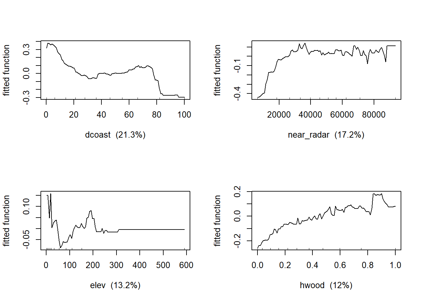
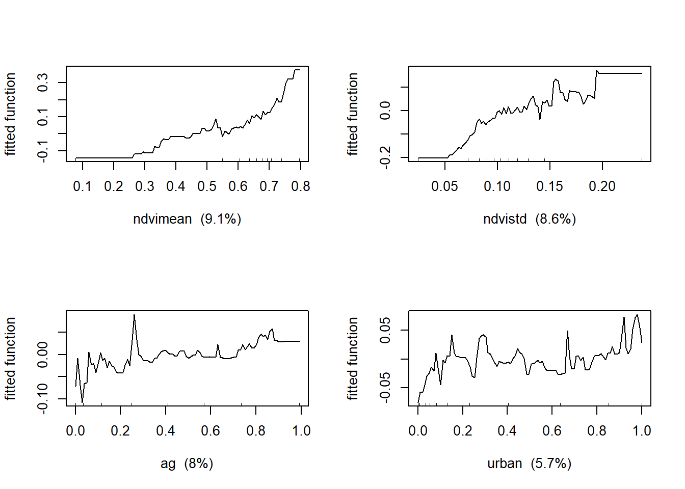
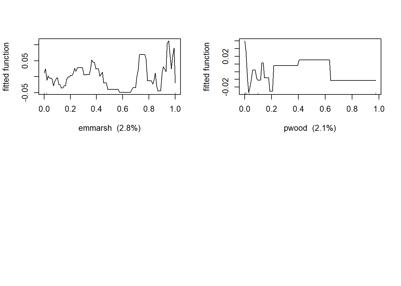
##                   var   rel.inf
## dcoast         dcoast 21.335562
## near_radar near_radar 17.178529
## elev             elev 13.207224
## hwood           hwood 11.989027
## ndvimean     ndvimean  9.106993
## ndvistd       ndvistd  8.568222
## ag                 ag  8.005161
## urban           urban  5.685826
## emmarsh       emmarsh  2.796909
## pwood           pwood  2.126548
The output shows the covariates ranked by their relative influence in explaning variance of the response variable. The relative influence among covariates will always add up to 100%. Look for the “cv correlation”. This is the cross-validation correlation.
7.1.0.1 Does it appear that the BRT models are informative?
Now let’s produce the partial dependency plots to see the functional responses between bird density and the predictor variables.
##If you model tree complexity >1 then look for interactions below
inter<-gbm.interactions(brt_model) #look for interactions among variables
## gbm.interactions - version 2.9
## Cross tabulating interactions for gbm model with 10 predictors## 1 2 3 4 5 6 7 8 9## $rank.list
## var1.index var1.names var2.index var2.names int.size
## 1 2 near_radar 1 elev 9.60
## 2 8 dcoast 2 near_radar 3.28
## 3 5 urban 2 near_radar 2.42
## 4 7 ndvistd 2 near_radar 2.03
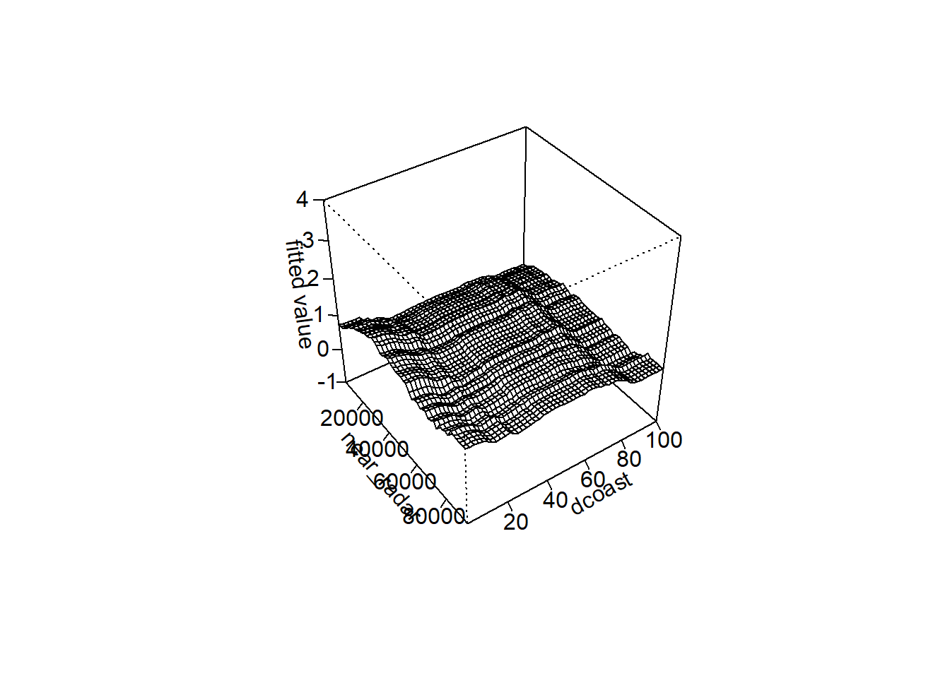
## 5 8 dcoast 4 hwood 1.87gbm.perspec(brt_model,2,8,z.range=c(-1,4)) #this function creates a perspective plot to visualize any interactions. Just replace the "2" and "7" with the index number of the two covariates you want to display## maximum value = 1.46