2 Basic visualization of radar scans

2.1 The structure of polar volumes

# Let's load a NEXRAD polar volume file for the KHGX radar (Houston):
my_pvol <- get_pvol("KHGX", as.POSIXct("2017-05-04 01:25:00"))

## Filename = /var/folders/85/mhhbjmj50wnb0_g0kntpzrw80000gr/T//Rtmpd0QsIA/KHGX20170504_012315_V0611df63f3584b5, callid = KHGX

## Removed 1 SAILS sweep.

## Call RSL_keep_sails() before RSL_anyformat_to_radar() to keep SAILS sweeps.

## Reading RSL polar volume with nominal time 20170504-012315, source: RAD:KHGX,PLC:HOUSTON,state:TX,radar_name:KHGX

# The default summary information of a `pvol` object contains information
# on the scans (sweeps) and their moments:
my_pvol

##                Polar volume (class pvol)
## 
##      # scans:  14 
##        radar:  KHGX 
##       source:  RAD:KHGX,PLC:HOUSTON,state:TX,radar_name:KHGX 
## nominal time:  2017-05-04 01:23:15

# We can also extract the elevation angles from the polar volume as follows:
get_elevation_angles(my_pvol)

##  [1]  0.483395  0.878910  1.318360  1.801755  2.416995  3.120115  3.999025
##  [8]  5.097660  6.416020  7.998050 10.019530 12.480470 15.600585 19.511719

2.2 Plotting radar scans

# let's extract the scan collected at 0.5 degree elevation from our polar volume:
my_scan <- get_scan(my_pvol, 0.5)
# print some information about this scan:
my_scan

##                   Polar scan (class scan)
## 
##      parameters:  DBZH RHOHV WRADH PHIDP ZDR VRADH 
## elevation angle:  0.483395 deg
##            dims:  1201 bins x 720 rays

# let's plot the reflectivity factor parameter of the scan in a range - azimuth coordinate system:
plot(my_scan, param = "DBZH")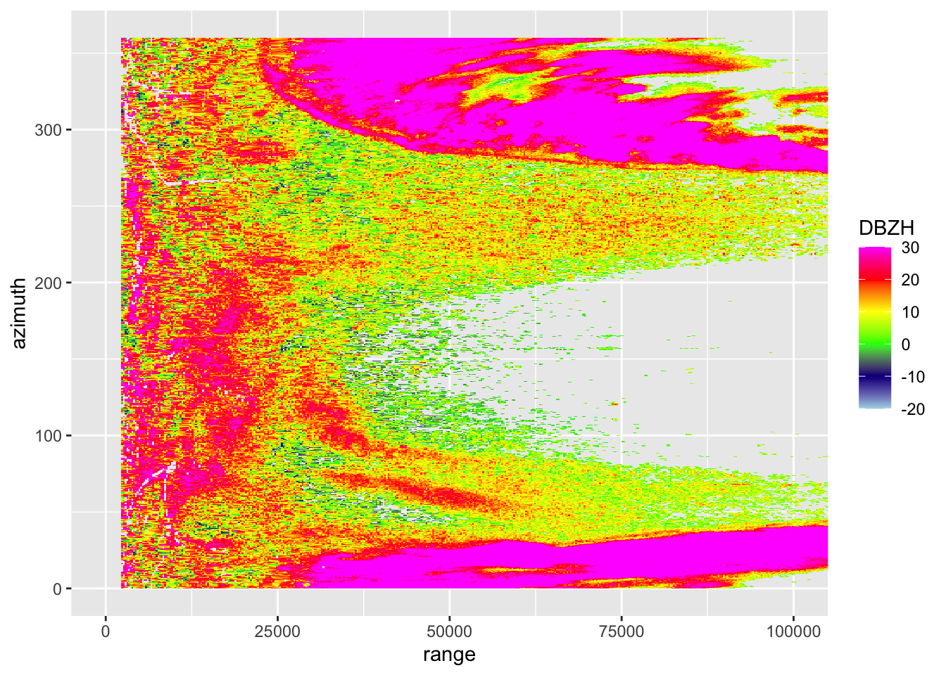

Exercise 1: Plot the radial velocity parameter (VRADH) of the 1.5 degree elevation scan in a range - azimuth coordinate system. (See manual page of the read_pvolfile() function for the nomenclature of various available quantities).

# Plot the radial velocity (VRADH) quantity of the 1.5 degree elevation scan:
plot(get_scan(my_pvol, 1.5), param = "VRADH")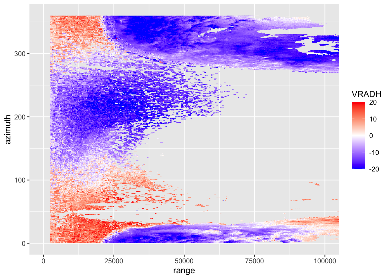

Often it is easier to visually explore radar scans as a PPI (plan position indicator), which is a projection of the scan on a Cartesian (X,Y) or (lat,lon) grid:

# before we can plot the scan, we need to project it on a Cartesian grid,
# i.e. we need to make a Plan Position Indicator (PPI)
my_ppi <- project_as_ppi(my_scan)
# print some information about this ppi:
my_ppi

##                Plan position indicator (class ppi)
## 
##   parameters:  DBZH RHOHV WRADH PHIDP ZDR VRADH 
##         dims:  201 x 200 pixels

# you can see we projected it on a 500 meter grid
# (check the manual of the project_as_ppi function to see how you can
# change the grid size (argument grid_size) and the maximum distance
# from the radar up to where to plot data (argument range_max))
#
# Now we are ready to plot the ppi, for example let's plot reflectivity factor DBZH:
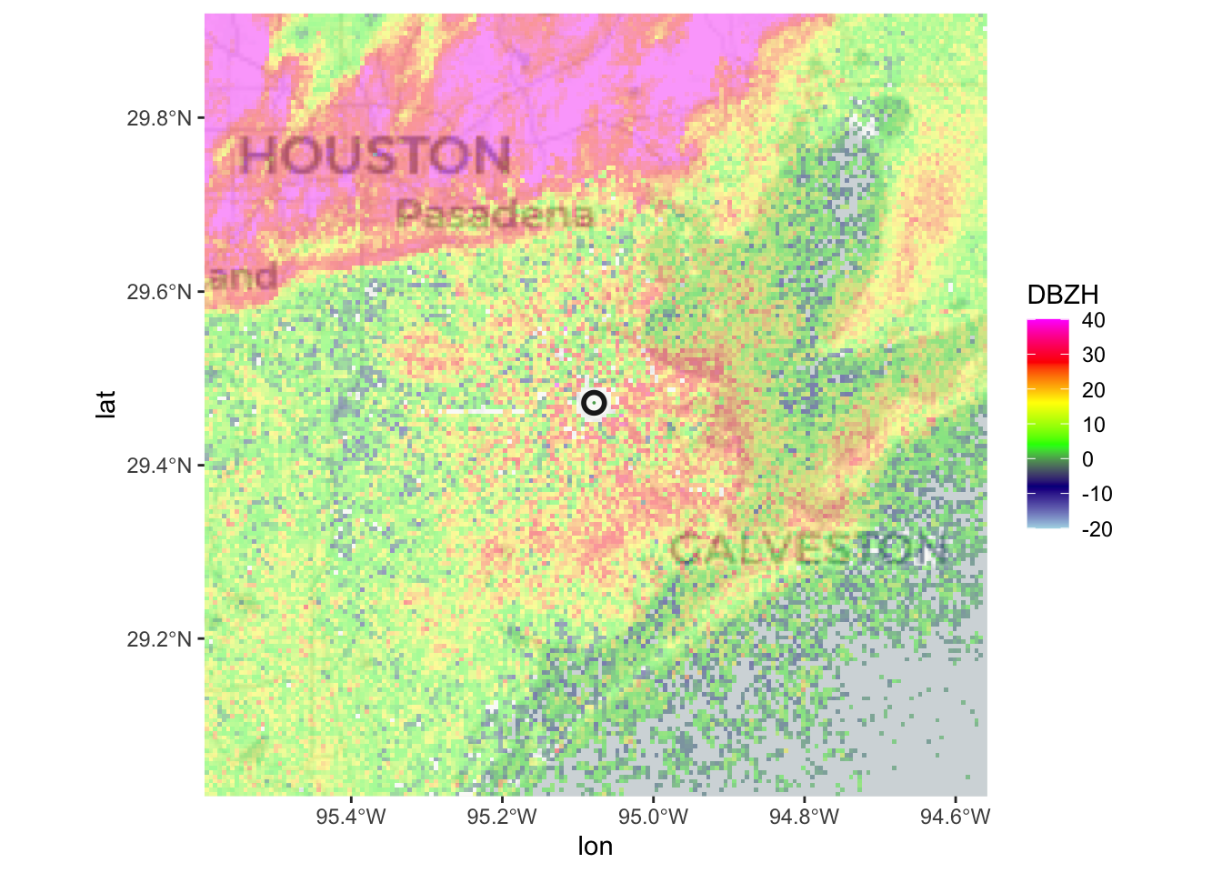
plot(my_ppi, param = "DBZH")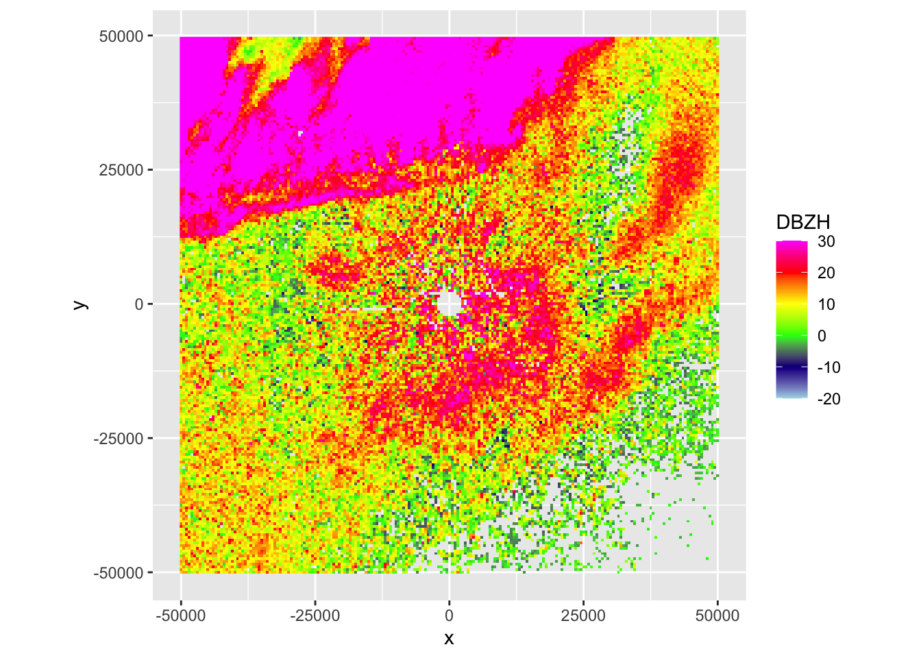

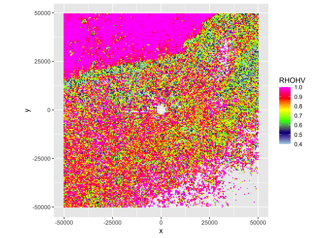
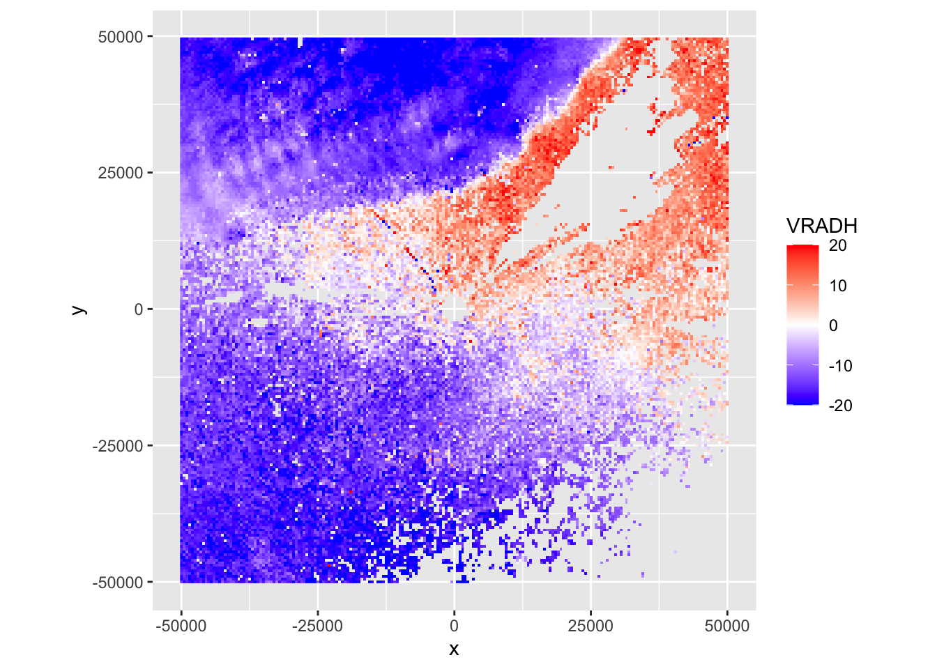
Exercise 2: This case shows an incoming precipitation front, characterized by localized but intense thunderstorms, as well as biological scattering. Make also a ppi plot of the correlation coefficient (RHOHV) and radial velocity (VRADH). Verify which regions are precipitation, and infer from those patterns the (approximate) direction of movement of biology and precipitation.

# Plot the correlation coefficient (RHOHV):
plot(my_ppi, param = "RHOHV")

# Plot the radial velocity (VRADH):
plot(my_ppi, param = "VRADH")

# Answer:
# * Precipitation areas are characterized by high correlation coefficients (typically > 0.95),
#   i.e. the top left corner of the image is precipitation
# * The blue radial velocity of the precipitation indicates it is moving towards the radar.
# * The radial velocity field of the biology shows areas south-west of the radar moving
#   towards the radar (blue), and areas north-east of the radar moving away from it (red).
#   The biology is therefore moving towards the north-east

Exercise 3: Based on the radial velocity image, are the biological scatterers birds or insects? Why?

# Answer:
# * Precipitation moves with the wind field. Since the biology moves into a different direction
#   than the wind and a very different speed, we can be sure these are birds.
#   The biological scatterers have a high self-propelled speed, which is
#   typical for birds, not for insects.

2.3 Overlaying radar scans on maps

# It is often informative to plot radar data on a base layer map.
# Function `bioRad::map`  overlays a PPI on a basemap (we restrict the color scale from -20 to 40 dBZ):
map(my_ppi, param = "DBZH", zlim = c(-20, 40), alpha=0.4)

## Zoom: 8