6 Processing many polar volumes
6.1 Accessing radar data
- US NEXRAD polar volume data can be accessed in the Amazon cloud. Use function
download_pvolfiles()for local downloads - European radar data can be accessed at https://aloftdata.eu. These are processed vertical profiles, the full polar volume data are not openly available for most countries. Data are available for single profiles (vp) in ODIM h5 format, or as monthly vertical profile time series (vpts) in VPTS CSV format.
- Use function
get_vpts()to download VPTS data from public repositories (aloft, birdcast, dark ecology). - Use function
get_pvol()to download polar volume data from public repositories (aloft, NEXRAD).
The names of the radars in the networks can be found here:
- US: NEXRAD network
- Europe: OPERA database
Useful sites for inspecting pre-made movies of the US composite are https://birdcast.info/migration-tools/live-migration-maps/ and https://www.pauljhurtado.com/US_Composite_Radar/.
6.2 Processing multiple polar volumes
This section contains an example for processing a directory of polar volumes into profiles:
It tends to be faster to first download a batch of files before processing them. Therefore we first we download files locally, and prepare an output directory for storing the processed profiles.
# First we download more data, for a total of one additional hour for the same radar:
# create a directory to store polar volumes (pvol data) and processed profiles (vp data)
dir.create("./data_pvol")
download_pvolfiles(date_min=as.POSIXct("2026-05-18 00:45:00"), date_max=as.POSIXct("2026-05-18 02:30:00"), radar="KBGM", directory="./data_pvol")
## Downloading data from unidata-nexrad-level2 for radar KBGM spanning over 1 days##
## Downloading pvol for 2026/05/18/KBGM/# We will process all the polar volume files downloaded so far:
my_pvolfiles <- list.files("./data_pvol", recursive = TRUE, full.names = TRUE, pattern="KBGM")
my_pvolfiles
# create output directory for processed profiles
outputdir <- "./data_vp"
dir.create(outputdir)We will use the following custom settings for processing: * We will use MistNet to screen out precipitation * we will calculate profile layers of 50 meter width * we will calculate 60 profile layers, so up to 5060=3000 meter altitude we will store the profiles in VPTS CSV format, by specifying an output file with extension .csv (this file format is fast for reading data back in later)
Note that we enclose the calculate_vp() function in tryCatch() to keep going after errors with specific files
Having generated the profiles, we can read them into R:
# we assume outputdir contains the path to the directory with processed profiles
my_vpfiles <- list.files(outputdir, full.names = TRUE, pattern="KBGM")
# print them
my_vpfiles
## [1] "./data_vp/KBGM20260518_003224_V06_vp.csv"
## [2] "./data_vp/KBGM20260518_003649_V06_vp.csv"
## [3] "./data_vp/KBGM20260518_004113_V06_vp.csv"
## [4] "./data_vp/KBGM20260518_004538_V06_vp.csv"
## [5] "./data_vp/KBGM20260518_005004_V06_vp.csv"
## [6] "./data_vp/KBGM20260518_005445_V06_vp.csv"
## [7] "./data_vp/KBGM20260518_005924_V06_vp.csv"
## [8] "./data_vp/KBGM20260518_010351_V06_vp.csv"
## [9] "./data_vp/KBGM20260518_010818_V06_vp.csv"
## [10] "./data_vp/KBGM20260518_011230_V06_vp.csv"
## [11] "./data_vp/KBGM20260518_011643_V06_vp.csv"
## [12] "./data_vp/KBGM20260518_012103_V06_vp.csv"
## [13] "./data_vp/KBGM20260518_012523_V06_vp.csv"
## [14] "./data_vp/KBGM20260518_012930_V06_vp.csv"
## [15] "./data_vp/KBGM20260518_013350_V06_vp.csv"
## [16] "./data_vp/KBGM20260518_013757_V06_vp.csv"
## [17] "./data_vp/KBGM20260518_014217_V06_vp.csv"
## [18] "./data_vp/KBGM20260518_014636_V06_vp.csv"
## [19] "./data_vp/KBGM20260518_015056_V06_vp.csv"
## [20] "./data_vp/KBGM20260518_015503_V06_vp.csv"
## [21] "./data_vp/KBGM20260518_015909_V06_vp.csv"
## [22] "./data_vp/KBGM20260518_020314_V06_vp.csv"
## [23] "./data_vp/KBGM20260518_020722_V06_vp.csv"
## [24] "./data_vp/KBGM20260518_021128_V06_vp.csv"
## [25] "./data_vp/KBGM20260518_021534_V06_vp.csv"
## [26] "./data_vp/KBGM20260518_021940_V06_vp.csv"
## [27] "./data_vp/KBGM20260518_022641_V06_vp.csv"## Registered S3 methods overwritten by 'readr':
## method from
## as.data.frame.spec_tbl_df vroom
## as_tibble.spec_tbl_df vroom
## format.col_spec vroom
## print.col_spec vroom
## print.collector vroom
## print.date_names vroom
## print.locale vroom
## str.col_spec vroom## Warning in validate_vpts(data): Extra fields found: height_reference
## Warning in validate_vpts(data): Extra fields found: height_referenceYou can now continue with visualizing and post-processing as we did earlier:
## Warning in plot.vpts(my_vpts, ylim = c(0, 3000)): Irregular time-series:
## missing profiles will not be visible. Use 'regularize_vpts' to make time series
## regular.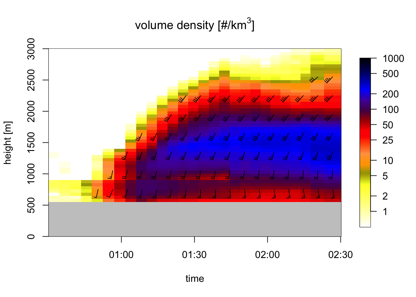
# let's visualize rain by plotting all aerial reflectivity:
plot(my_vpts, ylim = c(0, 3000), quantity="DBZH")
## Warning in plot.vpts(my_vpts, ylim = c(0, 3000), quantity = "DBZH"): Irregular
## time-series: missing profiles will not be visible. Use 'regularize_vpts' to
## make time series regular.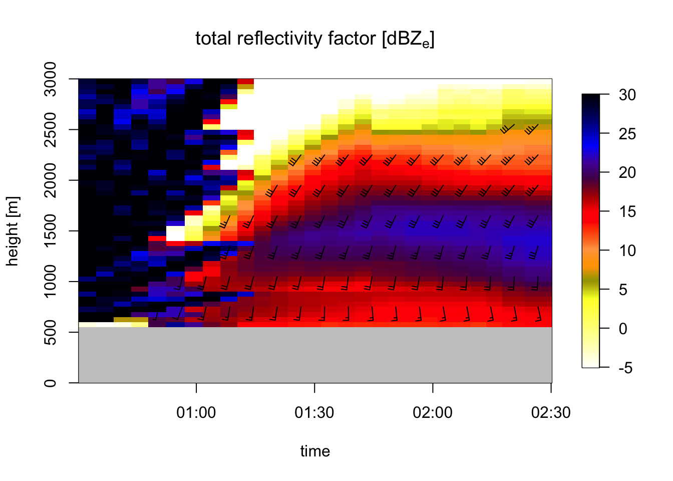 Note that we enclose the
 calculate_vp() function in tryCatch() to keep going after errors with specific files
6.3 Parallel processing
We may use one of the parallelization packages in R to further speed up our processing. We will use mclapply() from package parallel. First we wrap up the processing statements in a function, so we can make a single call to a single file. We will disable MistNet, as this deep-learning model does not parallelize well on a cpu machine.
process_file <- function(file_in){
  # construct output filename from input filename
  file_out <- paste(outputdir, "/", basename(file_in), "_vp.csv", sep = "")
  # run calculate_vp()
  vp <- tryCatch(calculate_vp(file_in, file_out, mistnet = FALSE, h_layer=50, n_layer=60), error = function(e) NULL)
  if(is.vp(vp)){
    # return TRUE if we calculated a profile
    return(TRUE)
  } else{
    # return FALSE if we did not
    return(FALSE)
  }
}

# To process a file, we can now run
process_file(my_pvolfiles[1])
## Filename = ./data_pvol/2026/05/18/KBGM/KBGM20260518_003224_V06, callid = KBGM## Reading RSL polar volume with nominal time 20260518-003224, source: RAD:KBGM,PLC:BINGHAMTON,state:NY,radar_name:KBGM## Running vol2birdSetUp## Warning: disabling single-polarization precipitation filter for S-band data, continuing in DUAL polarization mode## Warning in validate_vpts(data): Extra fields found: height_reference
## Warning in validate_vpts(data): Extra fields found: height_reference## [1] TRUENext, we use mclapply() to do the parallel processing for all files:
# load the parallel library
library(parallel)
# detect how many cores we can use. We will keep 2 cores for other tasks and use the rest for processing.
number_of_cores = detectCores() - 2
# Available cores:
number_of_cores
# let's loop over the files and generate profiles
start=Sys.time()
mclapply(my_pvolfiles, process_file, mc.cores = number_of_cores)
end=Sys.time()
# calculate the processing time that has passed:
end-start