6 Processing many polar volumes
6.1 Accessing radar data
- US NEXRAD polar volume data can be accessed in the Amazon cloud. Use function
download_pvolfiles()for local downloads - European radar data can be accessed at https://aloftdata.eu. These are processed vertical profiles, the full polar volume data are not openly available for most countries. Use function
download_vpfiles()for local downloads.
The names of the radars in the networks can be found here:
- US: NEXRAD network
- Europe: OPERA database
Useful sites for inspecting pre-made movies of the US composite are https://birdcast.info/migration-tools/live-migration-maps/ and https://www.pauljhurtado.com/US_Composite_Radar/.
6.2 Processing multiple polar volumes
This section contains an example for processing a directory of polar volumes into profiles:
First we download more files, and prepare an output directory for storing the processed profiles:
# First we download more data, for a total of one additional hour for the same radar:
download_pvolfiles(date_min=as.POSIXct("2017-05-04 01:40:00"), date_max=as.POSIXct("2017-05-04 02:40:00"), radar="KHGX", directory="./data_pvol")
## Downloading data from noaa-nexrad-level2 for radar KHGX spanning over 1 days##
## Downloading pvol for 2017/05/04/KHGX/# We will process all the polar volume files downloaded so far:
my_pvolfiles <- list.files("./data_pvol", recursive = TRUE, full.names = TRUE, pattern="KHGX")
my_pvolfiles
# create output directory for processed profiles
outputdir <- "./data_vp"
dir.create(outputdir)We will use the following custom settings for processing: * We will use MistNet to screen out precipitation * we will calculate profile layers of 50 meter width * we will calculate 60 profile layers, so up to 50*60=3000 meter altitude
Note that we enclose the calculate_vp() function in tryCatch() to keep going after errors with specific files
Having generated the profiles, we can read them into R:
# we assume outputdir contains the path to the directory with processed profiles
my_vpfiles <- list.files(outputdir, full.names = TRUE, pattern="KHGX")
# print them
my_vpfiles
## [1] "./data_vp/KHGX20170504_012843_V06_vp.h5"
## [2] "./data_vp/KHGX20170504_013405_V06_vp.h5"
## [3] "./data_vp/KHGX20170504_013934_V06_vp.h5"
## [4] "./data_vp/KHGX20170504_014502_V06_vp.h5"
## [5] "./data_vp/KHGX20170504_015031_V06_vp.h5"
## [6] "./data_vp/KHGX20170504_015600_V06_vp.h5"
## [7] "./data_vp/KHGX20170504_020127_V06_vp.h5"
## [8] "./data_vp/KHGX20170504_020656_V06_vp.h5"
## [9] "./data_vp/KHGX20170504_021224_V06_vp.h5"
## [10] "./data_vp/KHGX20170504_021752_V06_vp.h5"
## [11] "./data_vp/KHGX20170504_022320_V06_vp.h5"
## [12] "./data_vp/KHGX20170504_022848_V06_vp.h5"
## [13] "./data_vp/KHGX20170504_023417_V06_vp.h5"
## [14] "./data_vp/KHGX20170504_023946_V06_vp.h5"# read them
my_vplist <- read_vpfiles(my_vpfiles)You can now continue with visualizing and post-processing as we did earlier:
# make a time series of profiles:
my_vpts <- bind_into_vpts(my_vplist)
# plot them between 0 - 3 km altitude:
plot(my_vpts, ylim = c(0, 3000))
## Warning in plot.vpts(my_vpts, ylim = c(0, 3000)): Irregular time-series: missing
## profiles will not be visible. Use 'regularize_vpts' to make time series regular.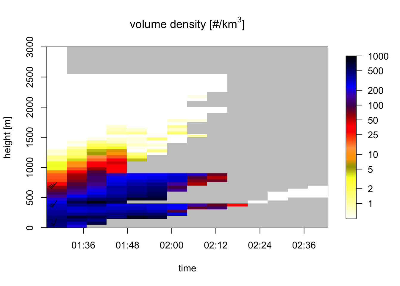
# because of the rain moving in, our ability to estimate bird profiles slowly drops:
# let's visualize rain by plotting all aerial reflectivity:
plot(my_vpts, ylim = c(0, 3000), quantity="DBZH")
## Warning in plot.vpts(my_vpts, ylim = c(0, 3000), quantity = "DBZH"): Irregular
## time-series: missing profiles will not be visible. Use 'regularize_vpts' to make
## time series regular.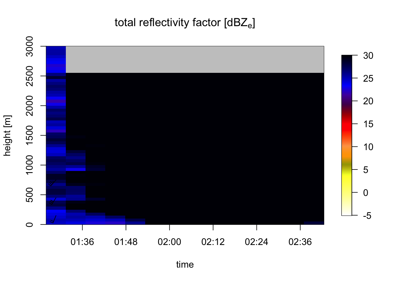 Note that we enclose the
 calculate_vp() function in tryCatch() to keep going after errors with specific files
6.3 Parallel processing
We may use one of the parallelization packages in R to further speed up our processing. We will use mclapply() from package parallel. First we wrap up the processing statements in a function, so we can make a single call to a single file. We will disable MistNet, as this deep-learning model does not parallelize well on a cpu machine.
process_file <- function(file_in){
  # construct output filename from input filename
  file_out <- paste(outputdir, "/", basename(file_in), "_vp.h5", sep = "")
  # run calculate_vp()
  vp <- tryCatch(calculate_vp(file_in, file_out, mistnet = FALSE, h_layer=50, n_layer=60), error = function(e) NULL)
  if(is.vp(vp)){
    # return TRUE if we calculated a profile
    return(TRUE)
  } else{
    # return FALSE if we did not
    return(FALSE)
  }
}

# To process a file, we can now run
process_file(my_pvolfiles[1])
## Filename = ./data_pvol/2017/05/04/KHGX/KHGX20170504_012843_V06, callid = KHGX
## Removed 1 SAILS sweep.
## Call RSL_keep_sails() before RSL_anyformat_to_radar() to keep SAILS sweeps.
## Reading RSL polar volume with nominal time 20170504-012844, source: RAD:KHGX,PLC:HOUSTON,state:TX,radar_name:KHGX
## Running vol2birdSetUp
## Warning: disabling single-polarization precipitation filter for S-band data, continuing in DUAL polarization mode## [1] TRUENext, we use mclapply() to do the parallel processing for all files:
# load the parallel library
library(parallel)
# detect how many cores we can use. We will keep 2 cores for other tasks and use the rest for processing.
number_of_cores = detectCores() - 2
# Available cores:
number_of_cores
# let's loop over the files and generate profiles
start=Sys.time()
mclapply(my_pvolfiles, process_file, mc.cores = number_of_cores)
end=Sys.time()
# calculate the processing time that has passed:
end-start