5 Range bias correction

In the previous section we have explored vertical integration of vertical profiles (vp’s). In this paragraph we will generalize vertical integration to entire radar images (ppi’s). To do that properly, we will account for the changing beam shape of the radar with range.

First, let’s examine the beam shape of the lowest elevation scan of the radar, which is typically around 0.5 degrees.

# define ranges from 0 to 2500000 meter (250 km), in steps of 100 m:
range <- seq(0, 250000, 100)

# plot the beam height of the 0.5 degree elevation beam:
plot(range, beam_height(range, 0.5), ylab = "beam height [m]", xlab = "range [m]", type='l')

# let's add the lower and upper altitude of the beam, as determined by the beam width:
points(range, beam_height(range, 0.5)-beam_width(range)/2, type='l',lty=3)
points(range, beam_height(range, 0.5)+beam_width(range)/2, type='l',lty=3)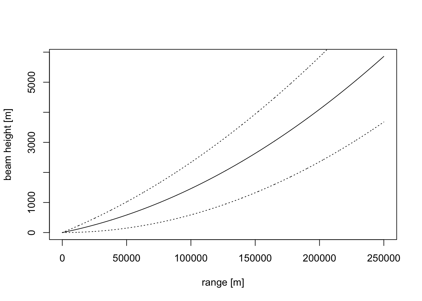

We will start with downloading a polar volume and processing it into a profile:

5.1 Processing a polar volume into a profile

# download a polar volume for the KBRO radar in Brownsville, TX
download_pvolfiles(date_min=as.POSIXct("2017-05-14 05:50:00"), date_max=as.POSIXct("2017-05-14 06:00:00"), radar="KBRO", directory="./data_pvol")

## Downloading data from noaa-nexrad-level2 for radar KBRO spanning over 1 days

## 
## Downloading pvol for 2017/05/14/KBRO/

# Load all the polar volume filenames downloaded so far for the KBRO radar:
my_pvolfiles <- list.files("./data_pvol", recursive = TRUE, full.names = TRUE, pattern="KBRO")
# we will process the first one into a vp:
my_pvolfile <- my_pvolfiles[1]
# calculate the profile, using MistNet to remove precipitation:
# we calculate 60 layers of 50 meter width, so up to 30*100=3000 m.
my_vp <- calculate_vp(my_pvolfile, n_layer=60, h_layer=50, sd_vvp_threshold = 1)

Exercise 13: Plot the bird density in the vertical profile you just estimated and compare it with the plots above of the beam height and width of the lowest radar beam. At which approximate range do you expect the radar will no longer be able to resolve the altitude distribution of the migratory birds. And at which range will the radar start to overshoot the migration layer entirely?

# plot the profile
plot(my_vp)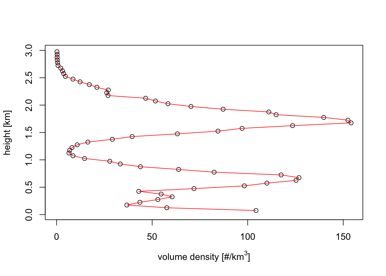

# Answer:
# * The vertical profile shows altitude bands of about 300 meter width
#   We therefore expect the radar to start having difficulty to resolve this profile
#   when the beam shape becomes broader, so at ranges less than 50 km
#   (this is why we typically use 35 km as the maximum range to use in vertical profile estimation.)
# * the birds fly up to about 2km in this profile.
#   At about 200000 m (200 km) the lower end of the beam no longer overlaps with the migration layer
#   Therefore, if we birds are flying according to the same altitude distribution everywhere,
#   we expect the radar to become fully blind for birds beyond 200 km

To correct for the decreasing ability of the radar to resolve the altitude distributions of birds with range, we will make one important (and likely imperfect!) assumption:

We assume that all birds within the image are distributed vertically according to the same relative vertical profile.

This assumptions simplifies the problem, and allows us to estimate the spatial distribution of the birds, as we will explore in the next paragraph:

5.2 Range bias correction and vertical integration on a map

# We will use the piping operator %>% of magrittr package to
# execute multiple operations in one statement:
library(magrittr)
# first, load the polar volume:
my_pvolfile %>% read_pvolfile() -> my_pvol

## Filename = ./data_pvol/2017/05/14/KBRO/KBRO20170514_055309_V06, callid = KBRO
## Reading RSL polar volume with nominal time 20170514-055309, source: RAD:KBRO,PLC:BROWNSVILLE,state:TX,radar_name:KBRO

# Next, let's calculate a PPI for the 1.5 degree elevation scan
# Finally, we calculated the vertically integrated PPI
my_ppi_integrated <- integrate_to_ppi(pvol=my_pvol,vp=my_vp, res=1000)

Exercise 14: Visually compare the PPI for the 1.0 degree sweep and the vertically integrated PPI, and explain the difference in spatial pattern. (For the clearest comparison, make plots of comparable parameters that are either linear or logarithmic in bird density).

# 
my_pvol %>%
  get_scan(elev = 1.0) %>%
  project_as_ppi(raster=raster::raster(my_ppi_integrated$data)) ->
  my_ppi
# let's take the logarithm of the vertically integrated density, so
# we can compare it more directly to DBZH, which is also a logarithmic quantity:
my_ppi_integrated <- calculate_param(my_ppi_integrated, logVID=log(VID))
# plot both ppi's:
plot(my_ppi)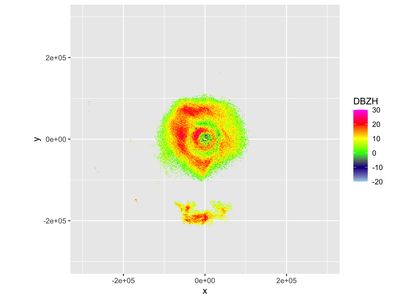

plot(my_ppi_integrated, param="logVID", zlim=c(-10,10))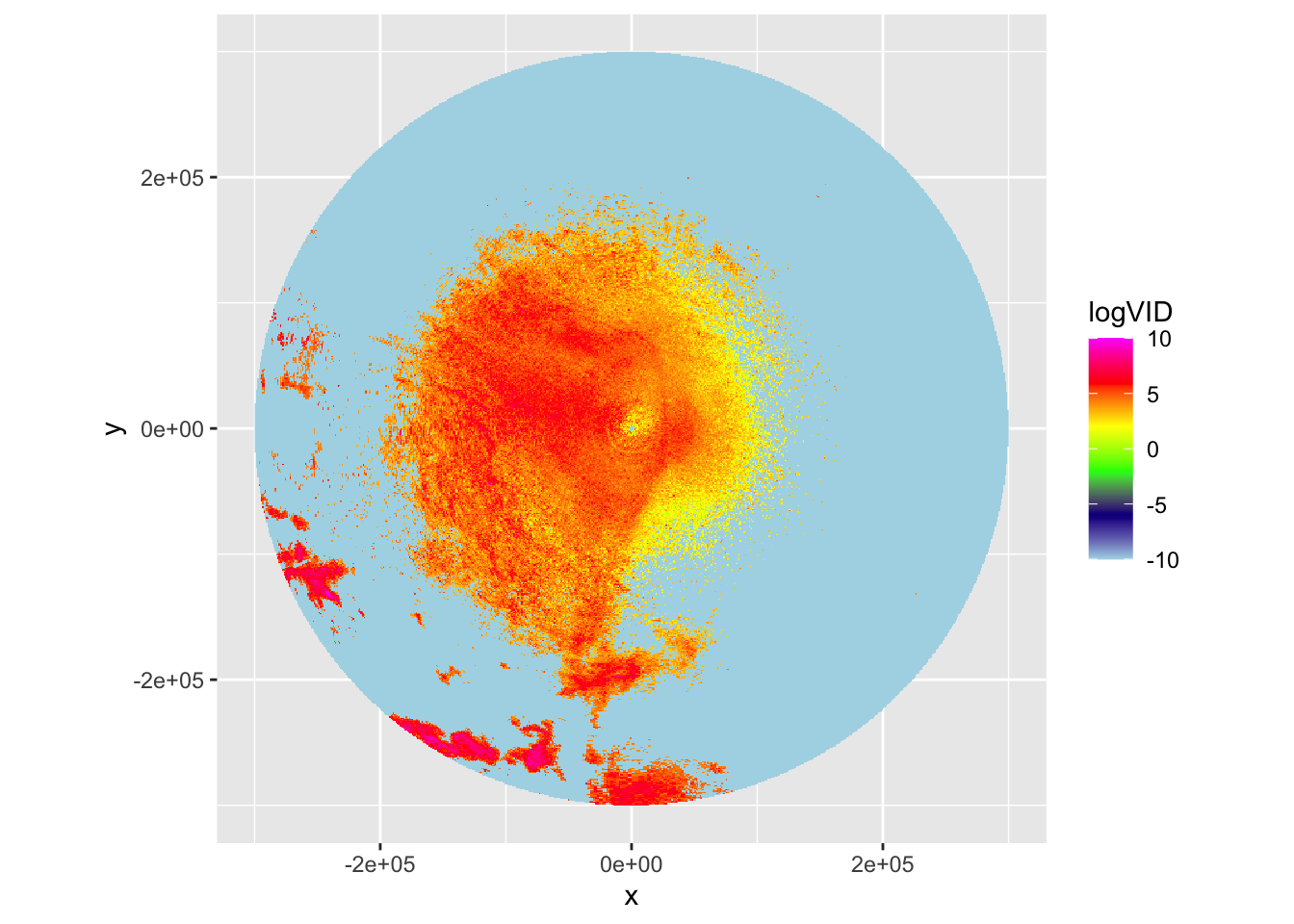

# The altitude distribution in this case shows two migration layers.
# In the 1.5 PPI scan these show up as two concentric rings of density.
# Since in a conventional PPI a larger distance from the radar also
# implies a higher altitude, we see the rings showing up at the
# ranges where the beam intersects each of the migration layers.
#
# The vertically integrated PPI is more straightforward to interpret
# Here we correct for aforementioned beam effects and integrate the
# density over altitude, giving a more realistic reconstruction of the
# spatial distribution of migrants.