3 Screening out weather
3.1 using correlation coefficient
Screening precipitation based on correlation coefficient is arguably the most simple and established approach for screening out weather in cases where dual-polarization data is available. It is based on removing data above a certain \(\rho_{/HV}\) tresholds, most commonly 0.95.
# We will screen out the reflectivity areas with for which the
# correlation coefficient is > 0.95 (indicating precipitation)
# We do so by redefining parameter DBZH, replacing pixels with NA values
# whenever RHOHV > 0.95
my_ppi_clean <- calculate_param(my_ppi, DBZH = ifelse(RHOHV > 0.95, NA, DBZH))
# plot the original and cleaned up reflectivity:
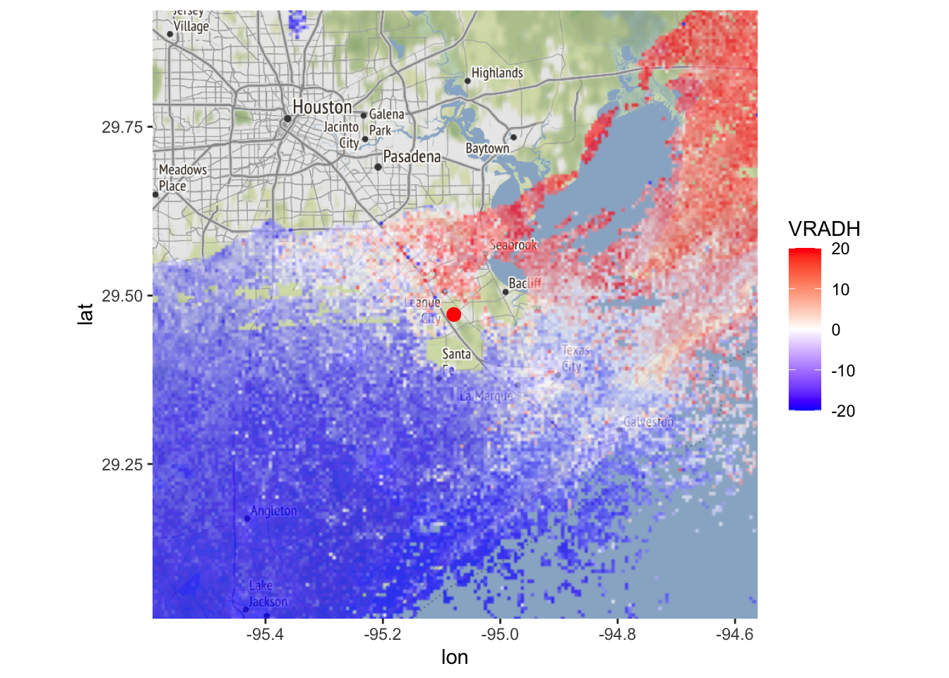
map(my_ppi, map = basemap, param = "DBZH", zlim = c(-20, 40))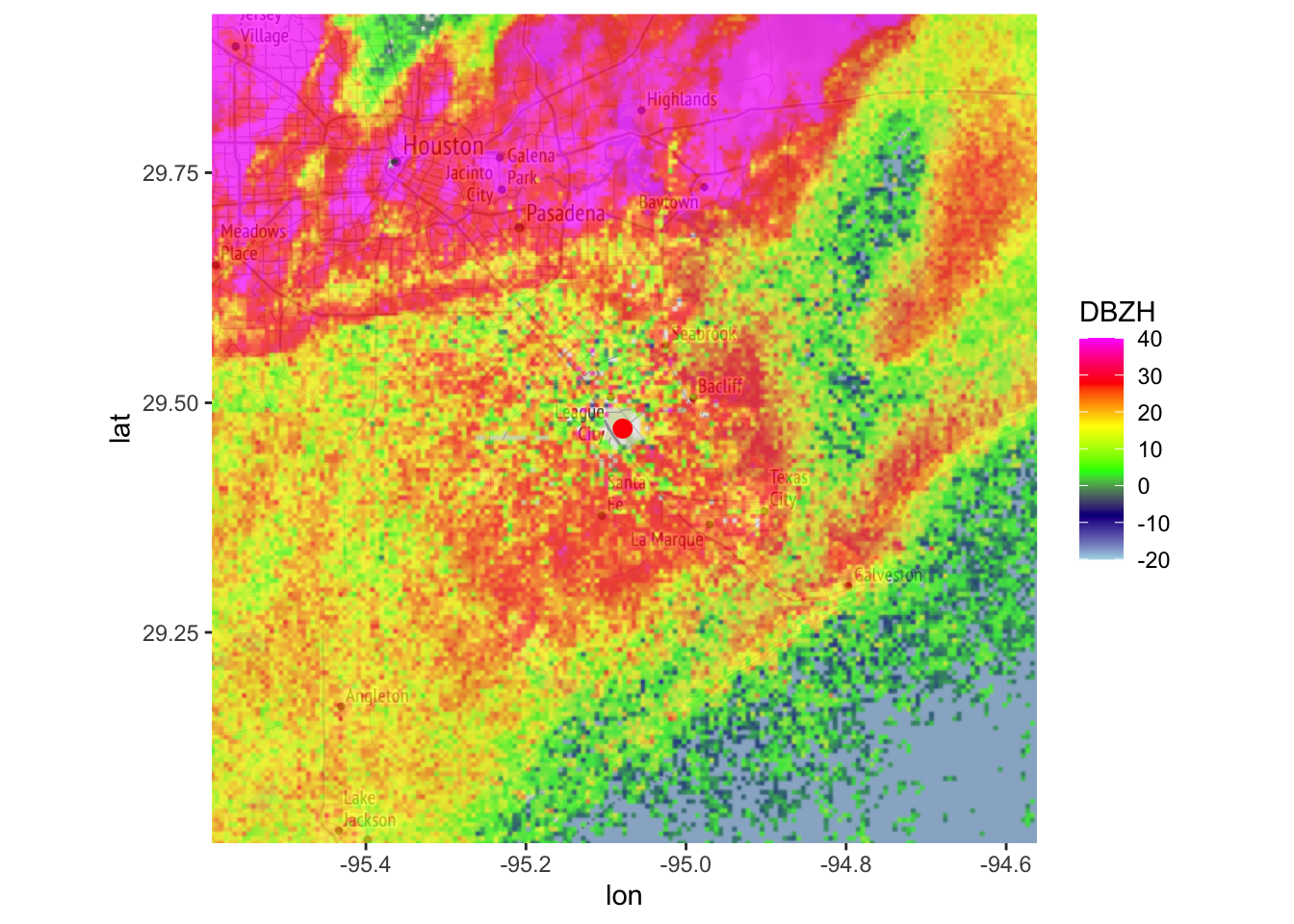
map(my_ppi_clean, map = basemap, param = "DBZH", zlim = c(-20, 40))
3.2 using MistNet
You can also use MistNet for screening out weather when * the radar operates at S-band wavelengths * you only have single polarization data available (specifically, the three basic quantities radial velocity VRADH, reflectivity DBZH, and spectrum width WRADH).
# apply the MistNet model to the polar volume file and load it as a polar volume (pvol):
my_pvol <- apply_mistnet(my_pvolfiles[1])
## Filename = ./data_pvol/2017/05/04/KHGX/KHGX20170504_012843_V06, callid = KHGX
## Removed 1 SAILS sweep.
## Call RSL_keep_sails() before RSL_anyformat_to_radar() to keep SAILS sweeps.
## Reading RSL polar volume with nominal time 20170504-012844, source: RAD:KHGX,PLC:HOUSTON,state:TX,radar_name:KHGX
## Running vol2birdSetUp
## Warning: disabling single-polarization precipitation filter for S-band data, continuing in DUAL polarization mode
## Warning: using MistNet, disabling other segmentation methods
## Running segmentScansUsingMistnet.
## Warning: Requested elevation scan at 1.500000 degrees but selected scan at 1.318360 degrees
## Warning: Requested elevation scan at 3.500000 degrees but selected scan at 3.120115 degrees
## Warning: Requested elevation scan at 4.500000 degrees but selected scan at 3.999025 degrees
## Warning: Ignoring scan(s) not used as MistNet input: 2 4 8 9 10 11 12 13 14 ...
## Running MistNet...done# mistnet will add additional parameters to the
# elevation scans at 0.5, 1.5, 2.5, 3.5 and 4.5 degrees
# let's extract the scan closest to 0.5 degrees:
my_scan <- get_scan(my_pvol, 0.5)
# plot some summary info about the scan to the console:
my_scan## Polar scan (class scan)
##
## parameters: DBZH VRADH RHOHV WRADH WEATHER BACKGROUND CELL PHIDP BIOLOGY ZDR
## elevation angle: 0.483395 deg
## dims: 1201 bins x 720 raysMistNet adds several new parameters:
WEATHER: a probability (0-1) for the weather classBIOLOGY: a probability (0-1) for the biology classBACKGROUND: a probability (0-1) for the background (empty space) classCELL: the final segmentation, which is based on the WEATHER parameters of all five MistNet elevation scans.CELLalso includes a border calculated by a region growing approach.CELLvalues equal 1 for the additional border, and 2 for the originally segmented precipitation area by MistNet.
# as before, project the scan as a ppi:
my_ppi <- project_as_ppi(my_scan)
# plot the probability for the WEATHER class
plot(my_ppi, param = 'WEATHER')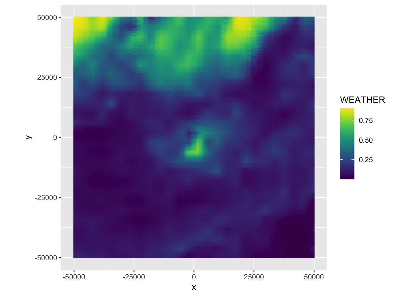
# plot the final segmentation result:
# plot the probability for the WEATHER class
plot(my_ppi, param = 'CELL')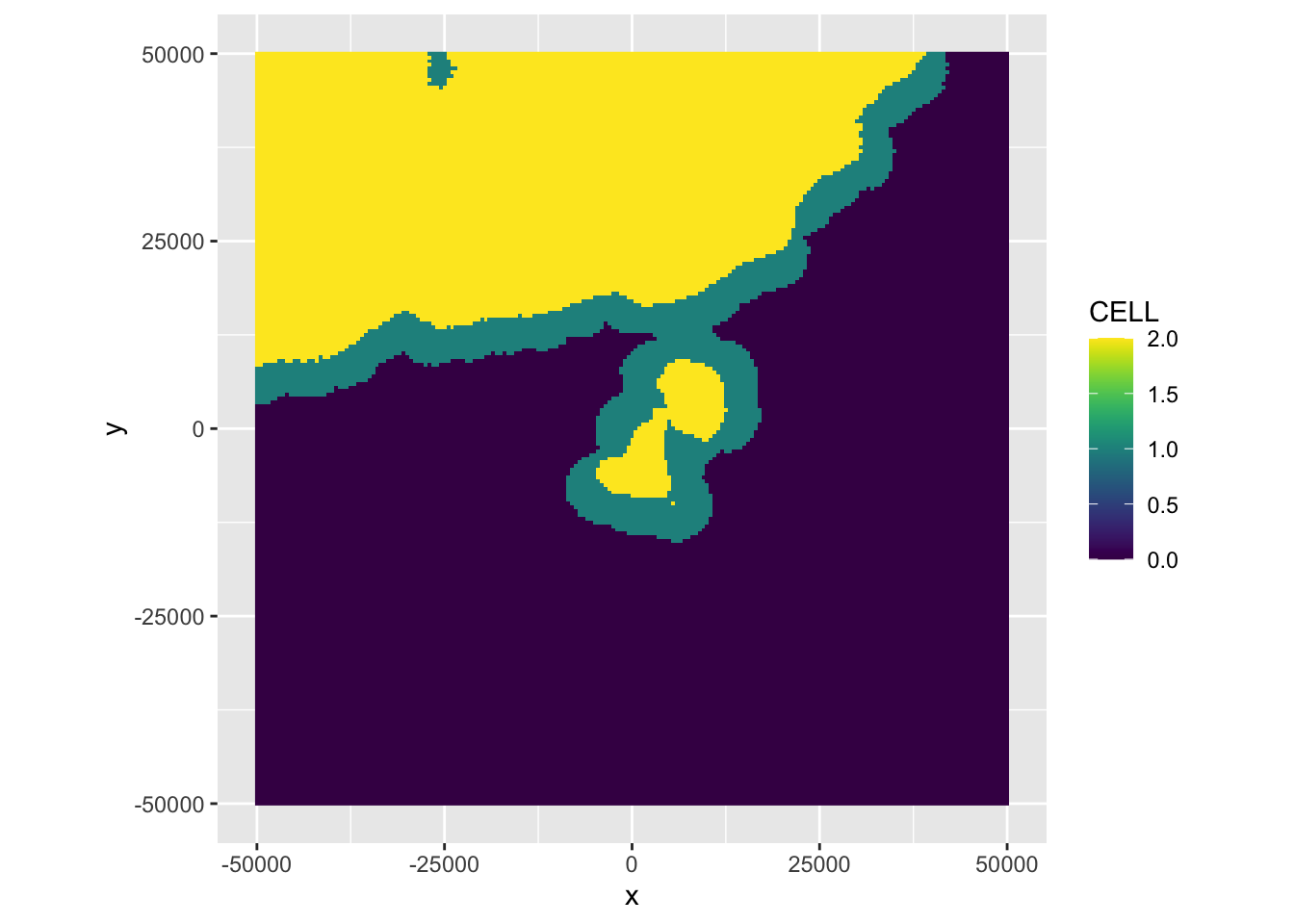
# let's remove the identified precipitation area (and additional border) from the ppi, and plot it:
my_ppi_clean <- calculate_param(my_ppi, DBZH = ifelse(CELL >= 1, NA, DBZH))
map(my_ppi_clean, map=basemap, param = 'DBZH')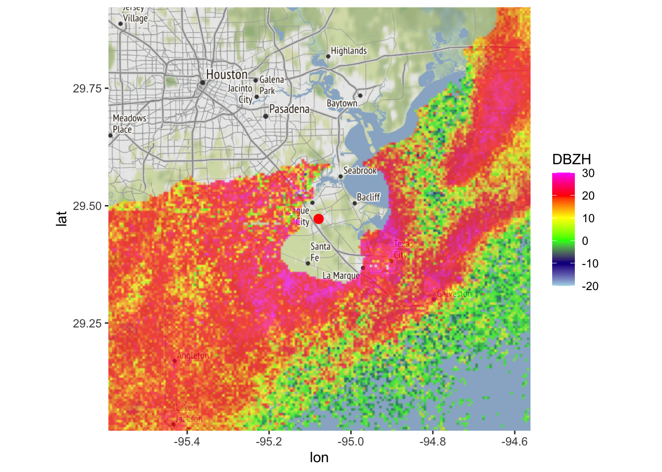
3.3 using depolarization ratio
Another quantity that has been proposed for distinguishing weather and biology is the depolarization ratio (\(D_r\)), which is defined as
\[D_r=\frac{Z_{DR}+ 1 -2 \sqrt{Z_{DR}} \ \rho_{HV}}{Z_{DR}+ 1 +2 \sqrt{Z_{DR}} \ \rho_{HV}}\] First we add the depolarization ratio (DR) as a parameter. We’ll express DR on a dB scale by transforming: \[DR=10\log_{10}(D_r) \] (see Kilambi et al. 2018, A Simple and Effective Method for Separating Meteorological from Nonmeteorological Targets Using Dual-Polarization Data for more information)
# let's add depolarization ratio (DR) as a parameter (following Kilambi 2018):
my_ppi <- calculate_param(my_ppi, DR = 10 * log10((1+ ZDR - 2 * (ZDR^0.5) * RHOHV) /
  (1 + ZDR+ 2 * (ZDR^0.5) * RHOHV)))
## Warning in eval(nn <- (calc[[i]]), x$data@data): NaNs producedLike correlation coefficient you can apply simple thresholds to its value to screen out precipitation. It has a good (potentially even better) ability to distinguish weather and biology:
  # plot the depolarization ratio, using a viridis color palette:
map(my_ppi, map = basemap, param = "DR", zlim=c(-25,-5), palette = viridis::viridis(100))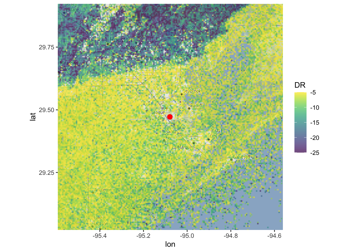
# Now let us screen out the reflectivity areas with DR < -12 dB:
my_ppi_clean <- calculate_param(my_ppi, DBZH = ifelse(DR < -12, NA, DBZH))
# plot the original and cleaned up reflectivity:
map(my_ppi, map = basemap, param = "DBZH", zlim = c(-20, 40))
map(my_ppi_clean, map = basemap, param = "DBZH", zlim = c(-20, 40))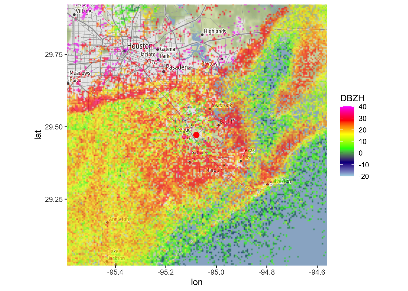
Exercise 4: Calculate and plot a ‘cleaned up’ PPI for the radial velocity that includes only the segmentation by MistNet and not the additional border. Remember that the segmentation by Mistnet has a CELL value 2, and the border has a CELL value 1.
# To remove the additional border around the rain segmentation by MistNet
# we want to screen out CELL values equal to 2 only.
my_ppi_clean <- calculate_param(my_ppi, VRADH = ifelse(CELL == 2, NA, VRADH))
map(my_ppi_clean, map=basemap, param = 'VRADH')